How to Use These Apps
Each app is designed to be explored interactively — provide inputs and observe the results in real time. The Hints & Tips below each app description explain the controls and suggest things to try. Some apps use your microphone for live audio input; your browser will ask permission when you activate that feature.
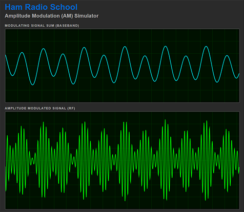
Simulates amplitude modulation of an RF carrier by a baseband signal such as audio. Provide your input and watch the carrier wave become amplitude-modulated in real time.
Adjusts the simulated RF carrier frequency and amplitude, and the apparent propagation speed of both baseband and carrier. Pauses waveforms and downloads a .png snapshot of the waveform displays.
Selects either an audio tone source as the modulating baseband or activates your microphone for live audio input.
The Modulating Signals (The Rack) allows you to add more sine waveforms that sum together into the modulating signal and produce more complex baseband waveforms. Each added sine wave can be adjusted in frequency and amplitude. Note: No audio tones are actually emitted — the simulated waveform of a pure sine wave is visually added to the modulating signal.
This option may require you to allow browser microphone access. Speak into your microphone to view real-time modulation of the complex audio baseband. Freeze the display during audio input for waveform analysis. Adjust the microphone gain to view effects of amplification.
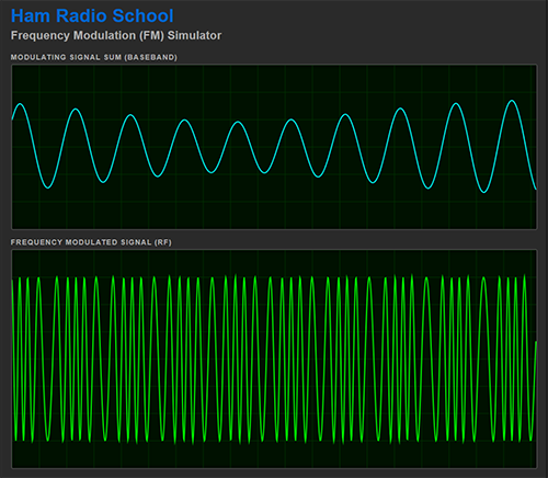
Simulates frequency modulation of an RF carrier by a baseband signal such as audio. Watch how audio input causes the carrier frequency to deviate above and below its center frequency.
Adjusts the simulated RF carrier frequency and amplitude, and the apparent propagation speed of both baseband and carrier. Pauses waveforms and downloads a .png snapshot of the waveform displays.
Selects either an audio tone source as the modulating baseband or activates your microphone for live audio input.
The Modulating Signals (The Rack) allows you to add more sine waveforms that sum together into the modulating signal and produce more complex baseband waveforms. Each added sine wave can be adjusted in frequency and amplitude. Note: No audio tones are actually emitted — the simulated waveform of a pure sine wave is visually added to the modulating signal.
This option may require you to allow browser microphone access. Speak into your microphone to view real-time frequency modulation of the complex audio baseband. Freeze the display during audio input for waveform analysis. Adjust the microphone gain to view effects of amplification.
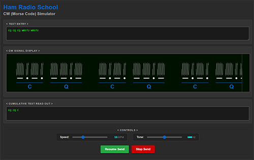
Simulates CW (Morse code) signals, translated from your input text. Enter text in the Text Entry field and click Start Send. The continuous waveform will flow across the display, underscored by the represented text characters.
Tones are emitted and the tone frequency can be adjusted with the lower right slider. Send speed can be adjusted, and the words per minute of the selected send speed is displayed. A cumulative text readout is also provided as the send proceeds.
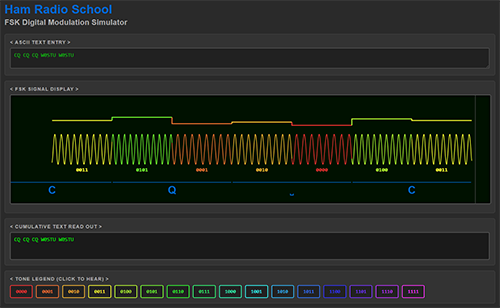
Simulates frequency shift keying encoded with standard 8-bit ASCII binary code. Enter text into the upper window and click Start Send. The FSK signal is represented in multiple forms simultaneously — audio tones, color-coded waveform, binary representation, stairstep function, and alphanumeric characters.
Select 2, 4, or 16 tone FSK. Note how the number of bits per tone symbol changes as the FSK type is changed.
Provides the color code and binary representation for each tone.
Adjusts the send speed. Zoom allows zooming in or out to view signal details and characters.
The baud is the symbols (individual tones) per second. The Data Rate is the bits per second. Note how the data rate increases even though the baud remains constant when you select a higher FSK type — each symbol represents a greater number of bits as the number of tones increases, making the code more efficient.
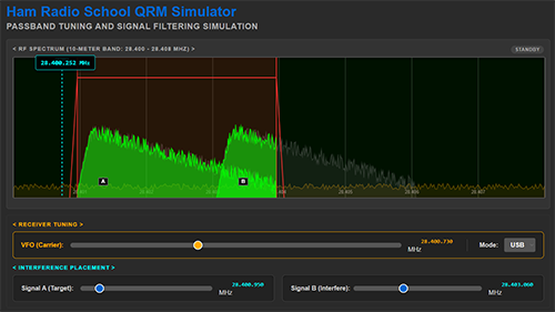
Simulates a receiver encountering QRM (man-made interference) in both Single Sideband (SSB) and Continuous Wave (CW) modes. Explore how adjustable bandwidth filtering can be used to isolate a target signal and reduce or eliminate nearby interfering signals, all visually depicted in an RF spectrum scope complete with audio effects.
Click the Start Receiver button to activate the received signals and associated sound. Adjust the VFO (Carrier) slider to tune your receiver to the target signal. Controls allow you to adjust the relative positions of the two signals in the band to create various interference scenarios.
Independent high-cut and low-cut frequency controls adjust the filter passband position and bandwidth relative to the VFO (carrier) frequency. Slicing off portions of an interfering signal visibly narrows the red passband and immediately muffles or completely eliminates the unwanted audio.
Switch between SSB (10-meter band) and CW (40-meter band) modes. The visual characteristics and bandwidth constraints change appropriately for the selected mode. Ultra-narrow filtering down to 100 Hz in CW mode and 500 Hz in SSB mode allows exploration of audio effects and isolation of signals.
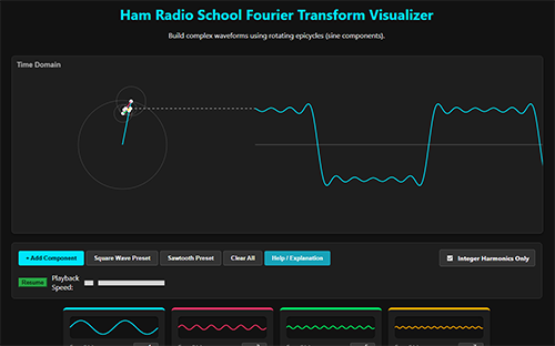
Illustrates how any complex signal can be constructed from individual sine wave components. Add together sets of linked rotating circles (epicycles), each representing a single sine wave component, to construct complex waveforms. Adjust amplitude, frequency, or phase of each to observe the effects.
Manually add up to eight sine wave components, or select presets to immediately construct a square wave or sawtooth wave. Observe the harmonic frequencies involved and manipulate components to observe skewing effects on these standard waveforms.
Start with the default single sine wave, then click "add component" to see odd integer harmonics of appropriate amplitude added in sequence to generate a square wave. Uncheck "integer harmonics only" to allow fractional harmonic multiples and observe how shifting, non-repeating complex waveforms can be constructed. Click "help / explanation" for additional insights.
Observe the constructed signal in a time-domain view or in a frequency-domain view, clearly visualizing how the summed component sine waves produce the complex waveform.
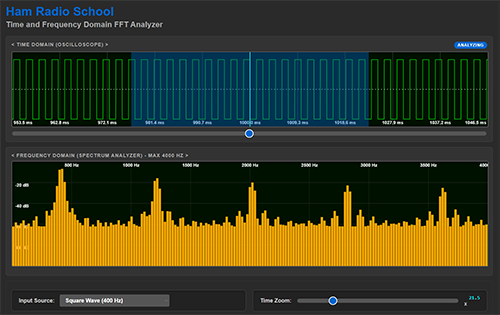
Illustrates the relationship between time domain signal representations and frequency domain representations. The lower frequency domain display is a spectrum analyzer view of the frequencies comprising the input signal, determined by fast Fourier transformation (FFT) of the blue-shaded window in the time domain (oscilloscope) display.
Select one of the pre-canned signal options or live microphone input. When using the microphone, click Start Microphone to activate and click again to record 2 seconds of audio.
Allows zooming for detailed analysis of the time domain view of the input.
Changes the number of discrete samples comprising the blue-shaded window in the time domain display. Greater numbers of samples provide greater resolution in the frequency domain display.
Select either a line graph or bar graph for the frequency domain display. The Play button plays the selected audio input. Reduce playback speed to get a slower playback — the tone will be preserved but slowed in time. Scroll down within the app to see a graphic illustrating the relationship between time domain and frequency domain views.
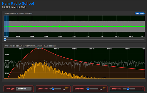
Illustrates the effects on audio signals of various filter types — simulating typical real-world (imperfect) filter effects. Similar interface to the FFT Analyzer, depicting both a time domain and frequency domain view with filter effects illustrated in the frequency domain display.
Select an input source (pre-canned signal or 5-second microphone recording). Select a filter type — a bandpass filter is recommended to begin. Adjust the Center Freq control to move the filter center frequency across the spectrum display.
Note the filter passband as the red-shaded region of the spectrum display. Frequencies outside the red-shaded region are filtered entirely, while the filter shape (red curve) proportionally shapes the frequency response within that region. The ghost display shows the unfiltered signal for comparison.
Adjust the bandwidth to broaden or narrow the filter across the spectrum. Adjust the sharpness and observe the effects on the filter skirt. Filter the spectrum and then play the audio to hear the impact. A loop function is provided for continuous playback of the audio.
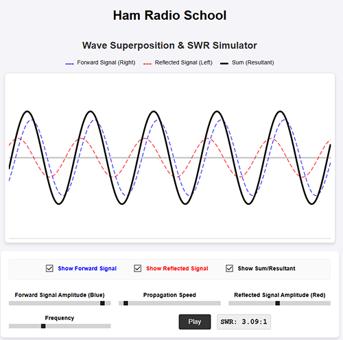
Illustrates the voltage traveling waveforms within a transmission line that can result in standing waves and increased SWR when an impedance mismatch is present. Select a forward signal amplitude, a reflected signal amplitude, propagation speed and a frequency.
A blue forward signal propagates left to right. A red reflected signal propagates right to left. A black summation of the two signals is computed and displayed — this is the standing wave.
Notice how the summation wave has a maximum voltage when the forward and reflected signals are in-phase (aligned), and a minimum voltage when they are exactly out of phase. SWR is computed as the ratio of maximum voltage to minimum voltage of the standing wave (black waveform) and is numerically displayed at the lower right.
Optionally turn each wave on or off with the check box selections. Pause the simulation as desired for analysis.
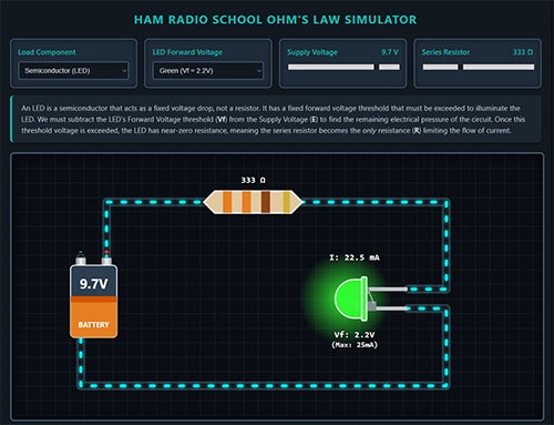
Illustrates a simple DC circuit containing a battery, one resistor, and either a filament lamp or an LED load. Make adjustments to the battery voltage or the series resistor value to visualize the change in current through the circuit and the impact on the LED or lamp.
The resistor displays color-coded stripes that change with the resistance value selected — just like a real resistor color code. Concise textual explanation is provided for each load type and calculation, making it easy to follow the math as you explore.
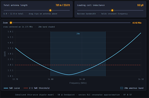
Illustrates the effects of dipole antenna modifications on SWR using a 20-meter band wire dipole example. Change the dipole length and observe the movement of the SWR curve up or down the band. Add inductive loading and see the SWR bandwidth narrow in response.
Intuitively grasp how trimming a dipole antenna tunes it to a desired portion of the band. Watch the SWR curve shift in real time as you adjust antenna length.
SWR curve, antenna diagram with length, loading coils with microhenries, resonant frequency with associated SWR, 2:1 SWR bandwidth and range, and feedpoint impedance.
Add inductive loading coils to the dipole and observe how the SWR bandwidth — or Q — narrows in response, giving you a hands-on feel for the tradeoffs in loaded antenna design.
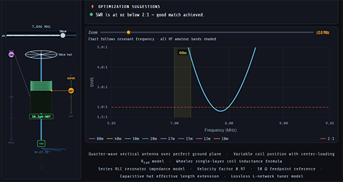
Adjust the vertical antenna element length to observe SWR curve movement across the RF spectrum from 80 meters to 10 meters. Simulate screwdriver antenna tuning by moving a wiper across loading coils to change inductive loading, and adjust coil position between base and mid-antenna.
Band presets automatically optimize all parameters for the selected band. When minimum SWR exceeds 2:1, the app provides specific optimization suggestions to guide the student.
Optionally apply a capacitive hat to the antenna and adjust its size for enhanced loading. Implement an antenna tuning network for tough matching scenarios. Observe the effects of each parameter on the SWR curve and feedpoint impedance in real time.
Based on a quarter-wave antenna with a perfect ground plane using the Wheeler coil inductance formula and a realistic radiative resistance model — perfect for illustrating the factors affecting loaded vertical antenna design.
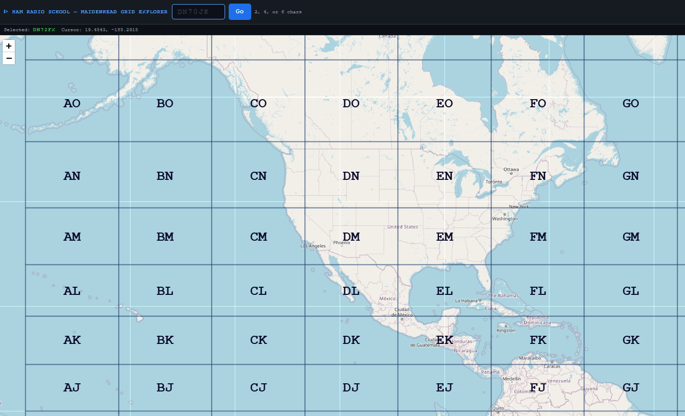
A visual Maidenhead Grid Locator system interactive mapper. Enter a known 2-, 4-, or 6-character Maidenhead Grid identifier and instantly find it anywhere on the globe.
Zoom, click and drag, or click grids to refine grid search or explore grid geography. Intuitive mouse-based and mobile responsive controls.
A geopolitical world map is overlaid with Maidenhead Locator System grids that change in resolution with your zoom level. Each grid in each level of resolution is outlined clearly and labeled with 2-, 4-, or 6-character ID. National, state, and city boundaries are depicted along with roadways and limited geographic terrain features.